In today’s post we’re going to talk about latencies in a common distributed system architecture: The root-leaf, or parent-child, fanout architecture. We’ll try to gain an intuition for what drives tail latency, derive a formula for tying together the parent and child latency distributions, and provide a useful interactive visualization to help understand tail latency in these systems.

Root-Leaf Fanout Architecture

When dealing with distributed systems, it’s a common pattern to have a root aggregator node that fans-out requests to many leaf nodes that do work in parallel, then send back their response to the root node to aggregate and create a final response. Usually the API of the system is exposed through the root-aggregator nodes, so the latency of these root nodes is what matters.

As seasoned distributed system developers, we know that latency (and performance) is a shape not a number. What this means is that we shouldn’t concern ourselves solely with what the average latency of a service is – we care about the full latency distribution – and at the very least we should care about the tail. Usually people settle on monitoring the \(90^{th}\) or \(99^{th}\) percentile (p90 or p99), and maybe use a heatmap to visualize the whole latency distribution.

In the case of our parent-aggregator and many children setup, if we’re going to concern ourselves with its p99 latency, it’d be nice to know for a given fanout, how fast do our children nodes have to be to get a certain p99 parent latency. This is also useful when debugging, but in reverse. If I see a p95 latency spike for the parent node, what percentile latency on the children nodes do I need to care about? How does this change with the fanout size?

Defining the Problem

Before we analyze the problem any further, we should first define exactly what problem we’re analyzing. In its simplest form, the parent-child system has two defining properties:

1. Parent latency for a request is greater than or equal to the max of all the children latencies, since the parent must wait for all child responses.
2. Child latency inevitably has a long tail.¹

These two properties mean that as we fan out to more children, our parent latency will get worse, because we’re more likely to hit a long tail latency event. And conversely if we can reduce our fanout or reduce the variance in our child latency we’ll be able to drive down our overall latency.

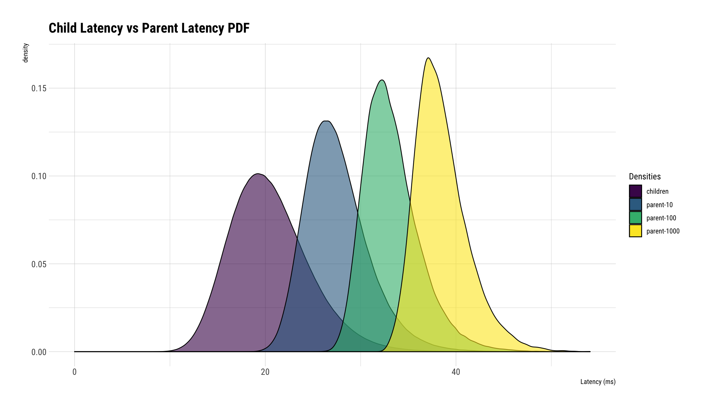
What’s not immediately obvious though is the magnitude of the effect of reducing fanout or improving child latency variance is. To try to gain some understanding, let’s consider a situation where the child latency follows a log normal distribution with \(\mu = 3\) and \(\sigma = 0.2\) and consider the latency distributions of the child, and parents who fan out to varying number of children per request: 10, 100, 1000.² Now we’ll visualize the reconstructed probability density functions based on observations from generated data, for both the children and the parents:

What’s immediately obvious is that as the fanout increases, the parent latency distribution gets worse and worse, and is dominated by the tail latency of the children. By the time we’re fanning out to 1000 children, the parent latency distribution looks almost completely unrelated to the child latency distribution. While we could have predicted this, hopefully this visualization helps build up our intuition of the problem.

Deriving a Closed Form Solution

We began this adventure trying to answer a question, and now it is time to return to it: What child latency percentile drives a given parent latency percentile?

Although the problem is pretty simple, I wrestled with it a bit until a friend pointed out that you can think of a percentile latency as not describing a point in the latency distribution but instead as a probability that a request finishes in a given amount of time. So if the p90 latency is 10ms, we can reframe this as saying that the probability a request finishes within 10ms is \(90\% \).

When we combine this insight with the fact that a parent request only finishes once all its children requests finish, we can derive a closed form solution to our problem.

Since the parent request finishes only after all \(N\) children requests finish, then the probability the parent request finishes in time \(t\), is the probability that all \(N\) children finish in time \(t\). Assuming all children latencies are independent and identically distributed³ then we can calculate the parent probability as:

$$ P_{parent\ finishes\ in\ t\ secs} = (P_{child\ finishes\ in\ t\ secs})^N $$

which when we solve for child latency percentile gives us the following formula:

$$ P_{child} \approx \sqrt[N]{P_{parent}} $$

Now that we have a formula for our problem, we can begin inspecting some secnarios. If we cared about the \(90^{th}\) percentile latency of the parent, and the fanout was to 2 children, then we would need to care about the \(94.86^{th}\) percentile at the children, since \(\sqrt{0.9} \approx 0.9486\).

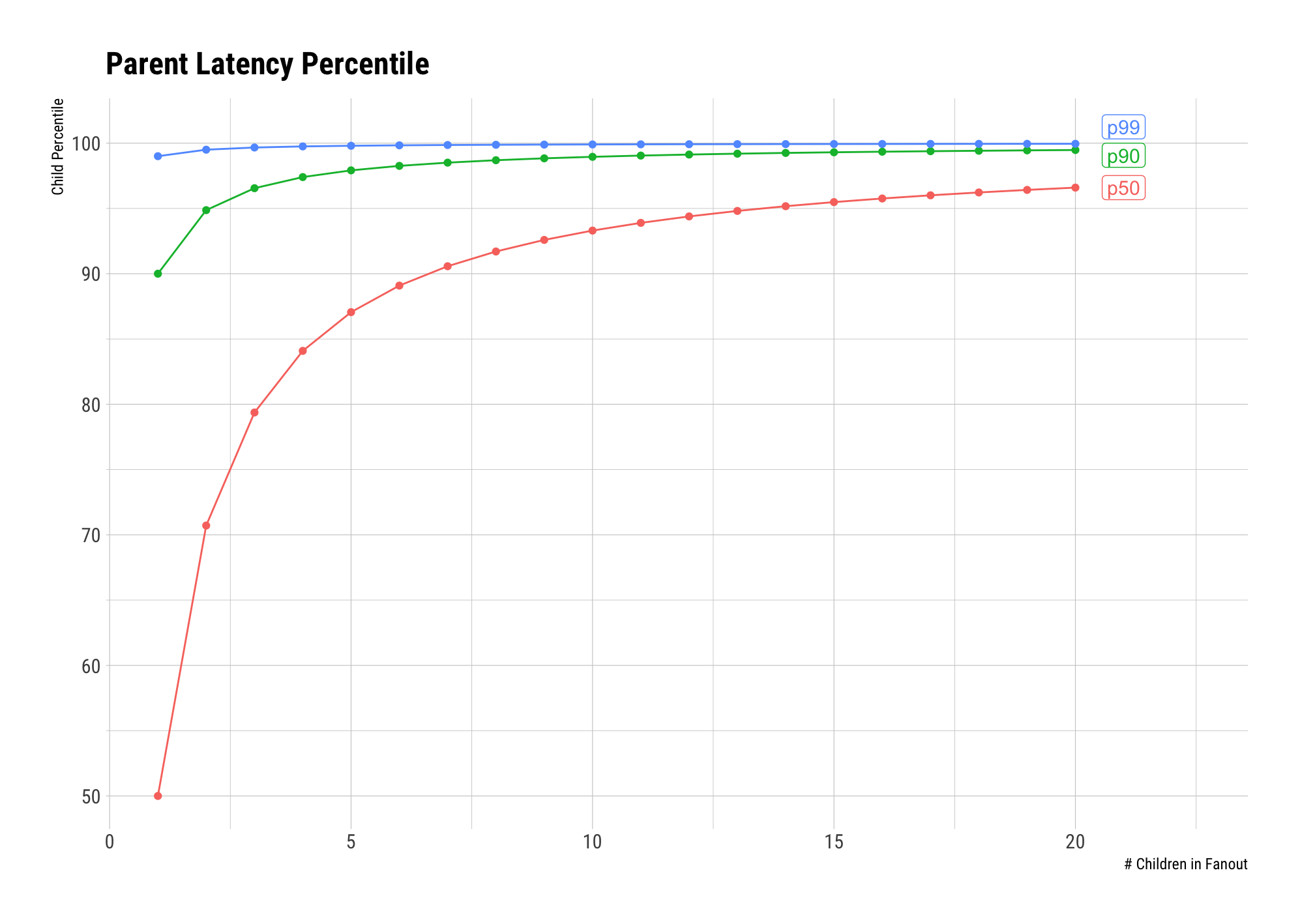
One thing about this formula that can be surprising, is how quickly the child percentile we have to care about grows as we increase the fanout. Even fanning out to 20 children, and monitoring the \(90^{th}\) percentile latency of the parent, we need to care about the \(99.47^{th}\) percentile latency of the children!

The graph below shows how quickly \(50^{th}\), \(90^{th}\), and \(99^{th}\) parent percentile latency converges to being driven by the \(100^{th}\) percentile child latency as fanout size grows.

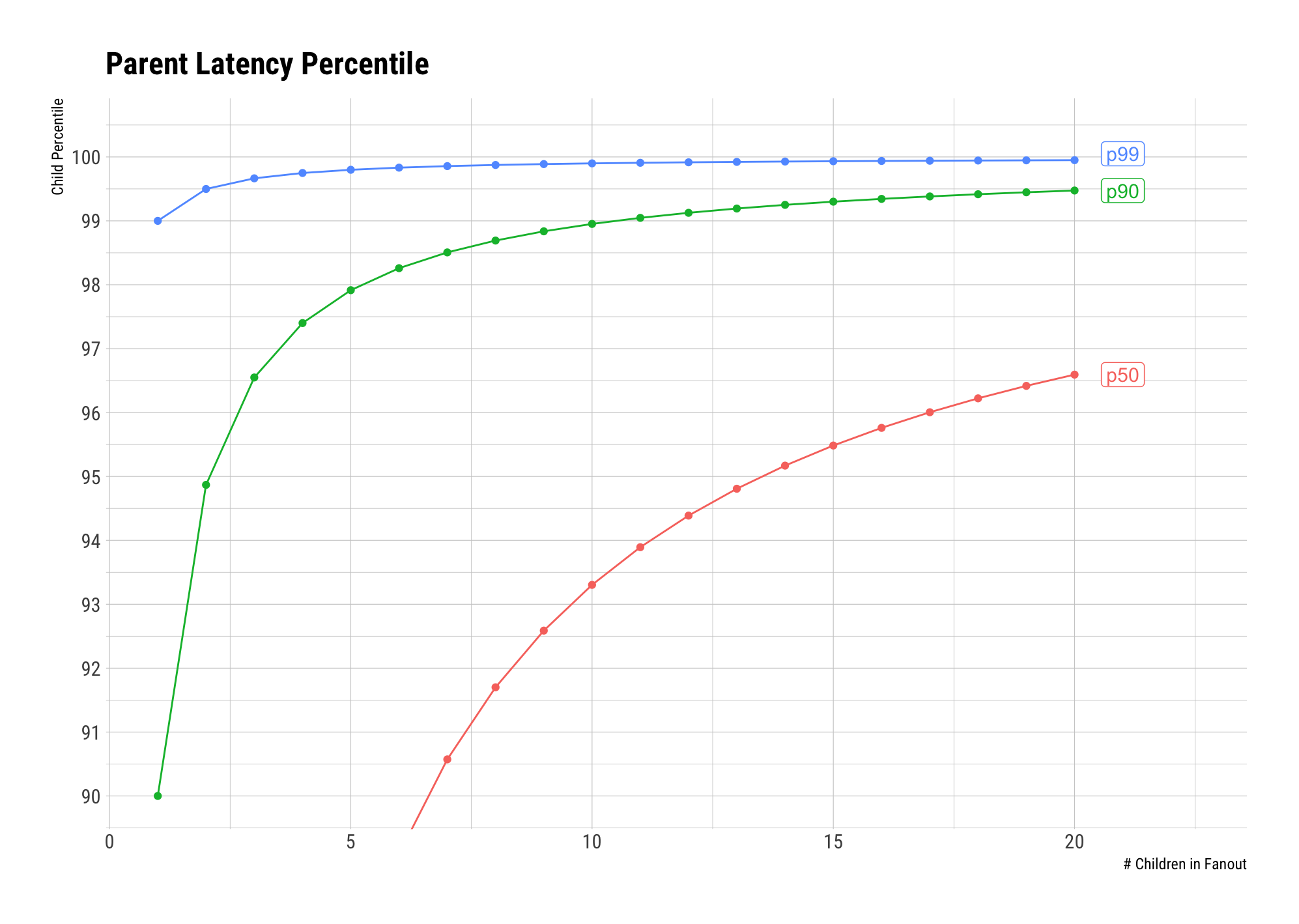
Here is a zoomed-in view focusing on the \(90^{th}\) percentile and above:

We can see that if we’re monitoring the p90 latency of the parent, by the time we fan out to 10 children, we’ll have to start caring about the p99 latency of the children.

Trust, but Verify (and Visualize)

Although the formula makes sense, and the intuition behind it sounds reasonable⁴, I often find it helpful when confronted with a formula to verify its correctness by simulation. So I below is a little simulation and visualization to do just that. The main spiffiness comes when you hover over a bar in either distribution, as the visualization will highlight both the percentile in its distribution as well as highlight the corresponding percentile in the other distribution:

The above is an example visualization generated from a generalized tool, simulating 3000 requests to a parent fanning out to 20 children, where the child latency distribution is a log normal distribution with \(\mu = 3.4\) and \(\sigma = 0.3\). The tool itself is hosted here, and the code is in this github repo.

Now we can use this visualization to confirm our formula empirically. If we hover over the bar that correlates with the p95 latency in the parent distribution, our formula predicts that the child latency it corresponds to should be \(\sqrt[20]{0.95} \approx .9974\) or p99.74, which is roughly what I get.

Bach’s Fanout Variations

While we now have a nice way to reason about and visualize the simplest version of the problem, there are still many variations that would be useful to understand.

Here are some things we might want to do to our system to improve the overall latency:

• What happens if we drop the slowest child request?
• What happens if we retry the slowest child request if it takes “too long”?
• What happens if we send every child request to two children instead and just use the fastest response?

I’m not the first person to think about this, lots of the ideas in this section are stolen directly from the Tail at Scale, as well as things I’ve observed in the wild.

This is a pretty rich topic, so hopefully in the future I can revisit it and update the visualization to take account of these subtleties.

Acknowledgements

Thanks to Jason for helping me with the formula, and thanks to Paul Khuong and Ray Yang for reading earlier drafts of this post.